
Can you Front-Run Institutional Rebalancing?
Inspired by The Unintended Consequences of Rebalancing


The Premise
While much of the research in modern markets has focused on persistent forces like momentum, value, or macro news, relatively little attention has been given to mechanical rebalancing.
In this post, we focus on one of the most well-known and widely implemented allocations: the 60/40 portfolio — 60% equities, 40% bonds. Specifically, we’re interested in what happens when that balance drifts and money managers are forced to rebalance.
The idea comes from “The Unintended Consequences of Rebalancing”, a paper by Campbell R. Harvey, Michele G. Mazzoleni, and Alessandro Melone (2025), which explores how predictable equity-bond rebalancing activity may create short-term price pressures and how those flows might be front-run or faded systematically.
We’re not going to attempt to replicate their results to the decimal point. This isn’t about academic fidelity. Instead, we’re using the paper as a launchpad — a way to identify and extract the core edge buried in the data. If that edge holds up, we’ll trade it. If not, we walk away. But the goal here isn’t replication for its own sake, it’s edge discovery for practical trading.
The Idea
At its core, this study explores whether we can position ourselves in S&P 500 futures (for equities) and 10-Year Treasury futures (for bonds) in such a way as to front-run the rebalancing activity of 60/40 portfolios.
That’s the hypothesis. Let’s extract the edge.
We will explore the rebalancing that can occur as a result of a :
Threshold-based signal — triggered when portfolio equity allocation has a significant weight deviation from 60 target.
Calendar-based signal — triggered at a certain time of the month such as end-of-month or quarter
These flows aren’t discretionary. They’re mechanical. That’s what makes them potentially tradable.
So our investigation begins with a simple question:
Can we anticipate and trade around these rebalancing signals using futures?
If either one reliably predicts equity-bond return spreads, we may be looking at a tradable edge.
The Edge
Let’s pause here, because this part matters.
The edge is everything.
It’s the foundation of any real trading strategy, it is the anomaly in the data that gives rise to alpha. Without it, a strategy is just a random set of rules. But once you extract an edge, you’ve got something you can structure a system around.
We’re not aiming for academic purity here. The data we use is different, and implementation requires some level of interpretation. What we are aiming for is simple: extract the edge the paper hints at, validate that it still exists, and then build rules to capture it.
We started with the threshold signal.
Threshold Signal
Definition: The Threshold Signal measures the deviation of the current equity holding from 60%. When the deviation goes over a certain threshold, the portfolio is rebalanced back to 60%.
Hypothesis: A negative signal today indicates an increase in the Equity-Bond spread the next trading day.
The logic behind the hypothesis is simple: a negative signal today means equities are underweight. To rebalance, traders will likely sell bonds and buy equities tomorrow, pushing the equity-bond spread higher.
So we need to regress the following equation to see if a relationship exists:

Before we begin our regression, we need to decide what threshold value (δ) to use to trigger a rebalance.
Rather than assume a specific threshold value, we take a more empirical approach — testing a range of values to see which levels produce a statistically significant predictive threshold signal.
We then regress each of these threshold signals against tomorrow’s equity–bond return spread to evaluate their predictive power.
Following the structure of the original paper, we test a range of δ values from 0% to 4%. The results are presented below.

The strongest t-stats appear in the range between 0% and 2% deviation — beyond that, the signal fades. This aligns with the intuition that rebalancing is more likely when the portfolio is slightly off target, but not excessively so.
Given we don’t want to use any particular threshold value, we build a new Average Threshold Signal, combining all threshold signals from 0% to 2%. This smooths out any individual noise and focuses on the region with the most consistent predictive value.
We then regress this average signal against next-day equity–bond return spreads to test we still have a statistically significant signal. The t-stat of -3.248 shows this Average Threshold Signal is even greater than the previous individual threshold signals.

This confirms that moderate equity-weight deviations in a 60/40 portfolio can reliably predict short-term return — providing us with a clean, tradeable signal.
When equities are underweight, the signal is negative → we expect equities to be bought tomorrow → the strategy goes long equities, short bonds.
Calendar Signal
Definition: The Calendar Signal captures the timing tendency of institutional rebalancing, based on the idea that many asset managers rebalance at fixed intervals. This signal measures the deviation of the equity allocation of a portfolio to the target 60% and rebalances on back to 60/40 on the last day of the month.
Hypothesis: A negative signal closer to month end indicates an increase in the Equity-Bond spread the next trading day.
The logic behind the hypothesis is institutions typically rebalance near month-end, so traders may begin front-running those flows in the final days of the month. We are looking for a negative calendar signal during these periods which suggests equity allocation is currently below 60%, and so expect equities will be bought and bonds sold, increasing the equity-bond spread tomorrow.
We test various rebalancing days towards the end of the month, using linear regression similar to what was performed for the Threshold Signal.
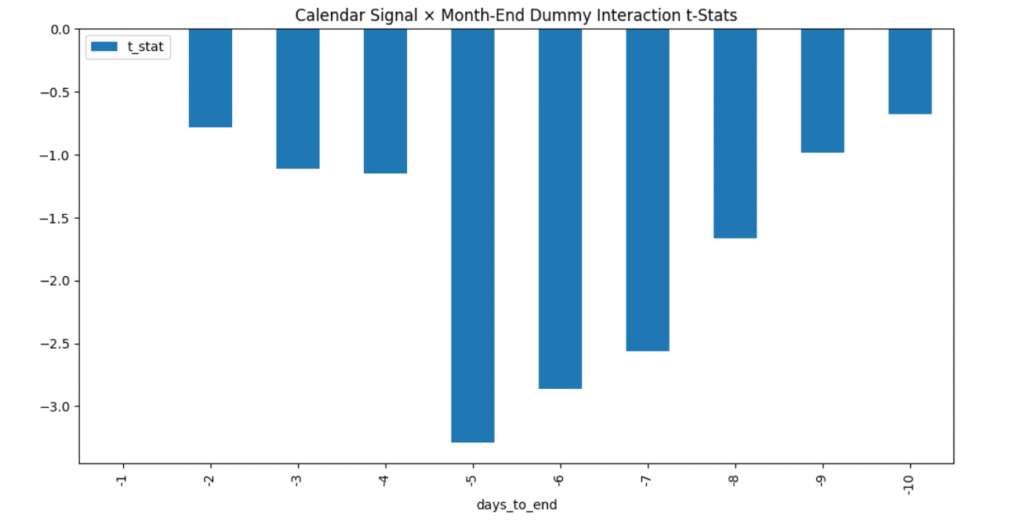
The chart above shows how strongly the calendar signal predicts the next day’s equity–bond return spread, based on how many trading days are left in the month. For example, if the x-axis shows “5,” we’re testing how predictive the signal is during the four trading days leading up to — but not including — the final day of the month. In other words, it’s five days to month-end, but we’re excluding the last day itself from the regression window. Why? Because by the final day, most of the rebalancing flows we’re trying to front-run have likely already hit. At that point, the edge flips. Instead of expecting more directional pressure, we’re often looking for a reversal. That’s why the last trading day isn’t part of the predictive window — it’s the day we use to position for mean reversion. As you’ll see in the strategy section, we assume that any forced buying or selling has mostly run its course by then. And like a coiled spring, prices are primed to snap back to their mean.
The Strategy
Now that we’ve shown both the threshold and calendar signals contain predictive power, it’s time to do something with them. Section 5 of the paper pulls it all together into a daily trading strategy, and we’re going to follow that structure.
The strategy trades the equity-bond spread — going long equities and short bonds (or vice versa) using futures, based on the strength of the combined signal. What this means is, the stronger the signal, the larger the weight of our spread position.
Here’s how it works: we first modify each of the signals, we then combine each of the modified signals together in a linear fashion, to create a single daily strategy weight. We then apply that weight to the equity-bond futures spread. Here’s the step-by-step breakdown:
Modified Threshold Signal
We take the Average Threshold Signal and make it usable in our strategy by rescaling it.
We convert it into the Modified Threshold Signal by simply dividing the output of the Average Threshold Signal by a normalization constant (0.012), and inverting the sign. We invert the sign since a negative signal implies a positive weight for the strategy (we discuss this more in the Position & Return Calculation section below).
Modified Calendar Signal
We take the Calendar Signal output and make the signal zero for all days accept for the last five trading days of each month. During the 4 days leading up to the final day of the month, we assign a value of -1 if the signal is positive and +1 if the signal is negative. On the final day of the month, after all the rebalancing price pressure has finished, we assign the inverse value to that of 5th last trading day of the previous month. We do this to position ourselves to take advantage of the expected mean reversion that happens during trading on the the first day of the month.
Combining the Signals into a Strategy Weight
Each of the signals discussed above captures a different source of rebalancing pressure and we combine them together to create a weight for our strategy:

This combined weight determines how aggressively we position in the equity-bond spread (long S&P 500 futures, short 10-year Treasury futures).
Position & Return Calculation
We take this strategy weight and apply it to the return difference between equity and bond futures:

A positive weight means we’re long equities, short bonds.
A negative weight means we’re long bonds, short equities.
A zero weight means we stay flat.
Before diving into the strategy mechanics, let’s first compare our equity curve to the one published in the original paper.


The resemblance is encouraging, our replication tracks the paper’s performance closely, which suggests we’ve captured the essence of the strategy well. With that validation in place, let’s move on to a deeper analysis of the results.
The below table shows the key performance statistics of the strategy compared to the SPY ETF which acts as a proxy to the S&P 500. We now scale the strategy to match the volatility of the SPY, and observe the equity curve of the strategy and it’s key statistics:
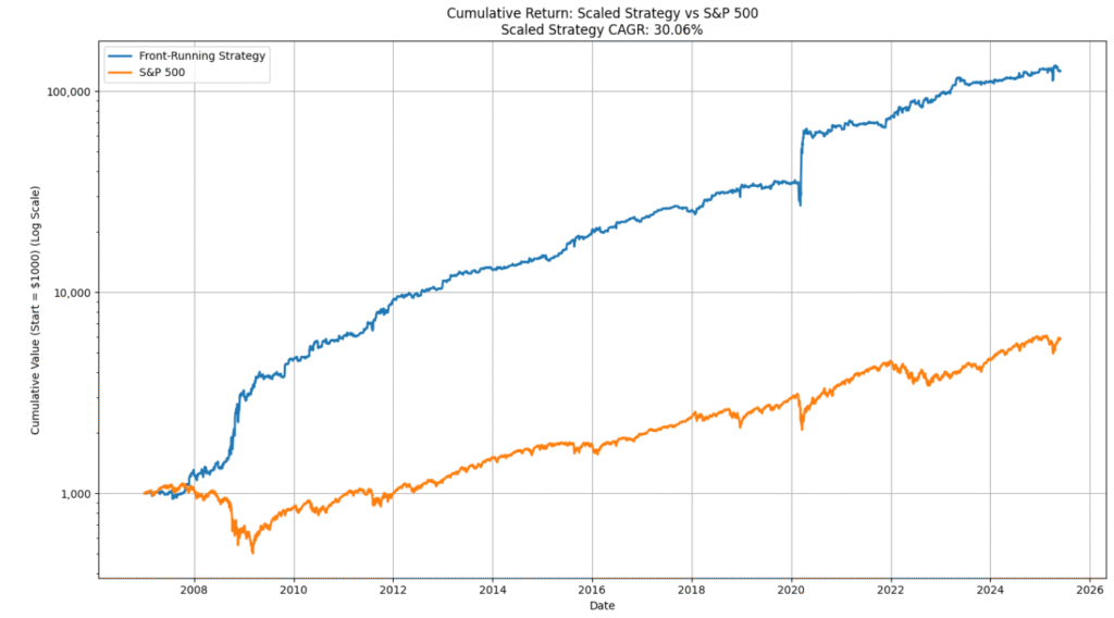

Even in the more recent period, the strategy continues to outperform on a risk-adjusted basis, with a Sharpe ratio more than double that of the S&P 500 and a remarkably low beta of 0.07. This suggests that the edge is still alive—and possibly still underexploited.
Notably, the strategy shows a Sharpe Ratio greater than 1.4 and a strong positive skew of 5.14, suggesting a tendency toward large upside outliers — a characteristic that enhances long-term compounding and is rarely found in high-Sharpe strategies.
Does the strategy work with ETF’s?
So far, the results suggest that this strategy, when implemented with futures, continues to perform well, even in today’s market. But the next natural question is: can this edge be captured using more accessible instruments like ETFs? To explore that, we tested the same approach using SPY (for equities) and TLT (for long-term bonds) as ETF proxies, which offer a practical path for implementation by a broader range of investors. Let’s take a look at how the strategy holds up when applied to these instruments.


Encouragingly, when applying the same strategy using ETFs like SPY and TLT, the results remained robust. Over the long run, the ETF-based version delivered a CAGR of 15.62% with a Sharpe ratio of 1.17, and still maintained the hallmark features of the futures-based strategy: low drawdown, low beta, and strongly positive skew (7.07). This suggests that even without futures, the underlying edge can still be accessed—making it far more practical for a wider range of investors.
Final Thoughts
This strategy doesn’t rely on forecasting fundamentals, chasing momentum, or reacting to news. Instead, it focuses on something simpler and arguably more persistent: predictable, mechanical flows.
By understanding when and why large allocators are forced to rebalance, we can position ahead of them, exploiting structural pressure without needing to predict the direction of the market.
It’s a strategy built not on opinion, but on observable behaviour and one that continues to show signs of strength.
Over the next few weeks, we’ll be spending some time adding this strategy to the QuantReturns.com strategy library, so you can track its daily performance.
In a future post, we’ll explore refinements, alternative signal weightings and potential ways to improve our results. But for now, the takeaway is clear:
Sometimes, knowing when someone else has to trade is the best edge you can have.
Disclaimer:
This article is for informational and educational purposes only. It discusses historical research and systematic strategies based on academic literature and does not constitute financial advice or a recommendation to buy or sell any security or investment product. All data and results presented are hypothetical and do not represent actual trading or investment performance. Past performance is not indicative of future results. Readers should conduct their own research and consult with a qualified financial professional before making any investment decisions.